Conflating Overture Places Using DuckDB, Ollama, Embeddings, and More

An Intro to Matching Place Data on Your Laptop
One of the trickiest problems in geospatial work is conflation, combining and integrating multiple data sources that describe the same real-world features.
It sounds simple enough, but datasets describe features inconsistently and are often riddled with errors. Conflation processes are complicated affairs with many stages, conditionals, and comparison methods. Even then, humans might be needed to review and solve the most stubborn joins.
Today we’re going to demonstrate a few different conflation methods, to illustrate the problem. The following is written for people with data processing or analysis experience, but little geospatial exposure. We’re currently experiencing a bit of a golden age in tooling and data for the geo-curious. It’s now possible to quickly assemble geo data and analyze it on your laptop, using freely available and easy-to-use tools. No complicated staging, no specialized databases, and (at least today) no map projection wrangling.
Further, the current boom in LLMs has delivered open embedding models – which let us evaluate the contextual similarity of text, images, and more. (Last year I used embeddings to search through thousands of bathroom fauces for our remodel.) Embeddings are a relatively new tool in our conflation toolkit, and (as we’ll see below) deliver promising results with relatively little effort.
We’re going to attempt to join restaurant inspection data from Alameda County with places data from the Overture Maps Foundation, enabling us to visualize and sort restaurants by their current inspection score.
And – inspired by the Small Data conference I attended last week – we’ll do this all on our local machine, using DuckDB, Ollama, and a bit of Python.
Sections
Staging the Data
First up, getting the data and staging it where we can work on it. Alameda County has its own data website where it hosts restaurant inspection records. We can see when it was updated (September 23rd, last week) and download the CSV. Go ahead and do that.
We need to get this CSV into a form where we can interrogate it and compare it to other datasets. For that, we’re going to use DuckDB. Let’s set up our database and load our inspections into a table:
Because we’ll need it later, I’m going to present all these examples in Python. But you could do most of this without ever leaving DuckDB.
Now we need to get Overture’s Places data. We don’t want the entire global dataset, so we’ll compute a bounding box in DuckDB that contains our inspection records to filter our request. We’ll take advantage of the confidence score to filter out some lower-quality data points. Finally, we’ll transform the data to closely match our inspection records:
We now have 56,007 places from overture and inspection reports for 2,954 foodservice venues.
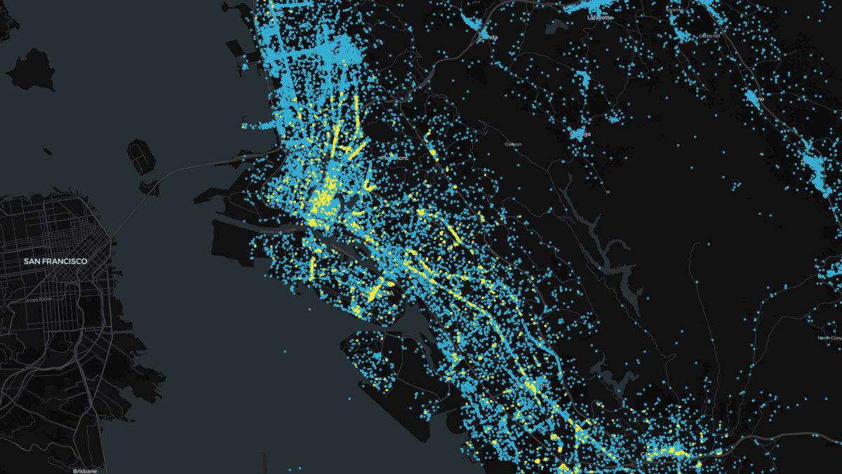
Looks good, but the blue points (the Overture data) go much further east than our inspection venues. Our bounding box is rectangular, but our county isn’t. If we were concerned with performance we could grab the county polygon from Overture’s Divisions theme, but for our purposes this is fine.
Generating H3 Tiles
In each conflation method, the first thing we’ll do is collect match candidates that are near our input record. We don’t need to compare an Alameda restaurant to a listing miles away in Hayward. We could use DuckDB’s spatial extension to calculate distances and filter venues, but it’s much easier to use a tile-based index system to pre-group places by region. Tile indexes aren’t perfect – for example, a restaurant could sit on the edge of tile – but for most matches they’ll work great.
We’re going to use H3 to tile our venues, because it’s fast and it has a DuckDB community extension so we don’t even have to bounce back up to Python. (Also, I ran into Isaac Brodsky, H3’s creator, at the Small Data conference. So it’s on theme!)
We’re now ready to try some matching. To sum up:
- We have two tables:
inspectionsandplaces. - Each has a
Facility_Name,Address,City,Zip,Longitude,Latitude, andh3column. These columns have been converted to uppercase to facilitate comparisons. - The Overture
placestable also has acategoriescolumn with primary and alternate categories. It might come in handy. - The
inspectionstable has aGradecolumn for each inspection, containing one of three values:Gfor green,Yfor yellow, andRfor red. Meaning ‘all good’, ‘needs fixes’, and ‘shut it down’ – respectively.
Let’s step through several different matching methods to illustrate them and better understand our data.
Method 1: Exact Name Matching
We’ll start simple. We’ll walk through all the facilities in the inspection data and find places within the same H3 tile with exactly matching names:
Inspecting the results, we matched 930 facilities to places. About ~31%, not bad!
We included the address columns so that when we scan these matches (and you always should, when building conflation routines), we can see if the addresses agree. Out of our 930 matched records, 248 have disagreeing addresses – or 26%. Taking a look, we see two genres of disagreement:
- The
placestable doesn’t capture the unit number in the address field. For example,BOB'S DISCOUNT LIQUORis listed as having an address of7000 JARVIS AVE, but has an address of7000 JARVIS AVE #Ain theinspectiondata.
This isn’t a problem, for our use case. We’re still confident these records refer to the same business, despite the address mismatch.
- Chain restaurants – or other companies with multiple, nearby outlets – will incorrectly match with another location close enough to occur in the same H3 tile. For example, a “SUBWAY” at
20848 MISSION BLVDis matched with a differentSUBWAYin the Overture data at791 A ST.
This is a problem. We used a resolution of 7 when generating our H3 tiles, each of which has an average area of ~5 km. Sure, we could try using a smaller tile, but I can tell you from experience that’s not a perfect solution. There are a shocking amount of Subways (over 20,000 in the US alone!), and plenty of other culprits will spoil your fun1.
We’ll need to solve this problem another way, without throwing out all the correctly matched venues from point 1 above.
Method 2: String Similarity
To find very similar addresses, we’ll use string distance functions, which quantify the similarity of two strings. There are plenty of different distance funcitons, but we’re going to use Jaro-Winkler distance because it weights matching at the beginning of strings more highly – which well suits our missing address unit situation. And hey, it’s built into DuckDB!
String distance functions produce a score, from 0 to 1, so we’ll have to figure out a good cut-off value. Let’s plot the distribution of the scores to get an idea:
Which produces:
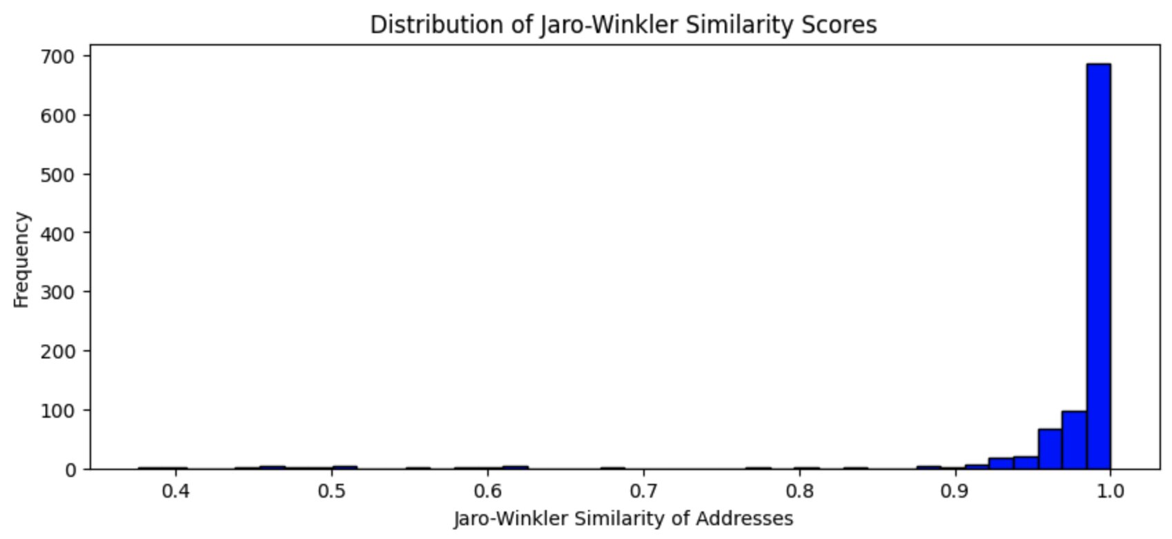
This looks super promising. Cracking open the data we can see the low scores are catching the nearby chain pairs: Subway, McDonald’s, Peet’s Coffee, etc. There are a couple false negatives, but we can solve those with another mechanism. Everything above a score of 0.75 is perfect. So our query looks like:
Which produces 903 matches we trust.
But what if we use Jaro-Winkler (JW) string distance to find very similar venue names, not just exact matches? Looking at the scores for similar names (where the venues share the same H3 tile and have addresses with a score of 0.75) we see the algo spotting the same venues, with slightly different names. For example, the inspections dataset often adds a store number to chain restaurants, like, CHIPTLE MEXICAN GRILL #2389. JW matches this strongly with CHIPOTLE MEXICAN GRILL. Everything above a score of 0.89 is solid:
This produces 1,623 confident matches, or 55%.
But looking at our potential matches, there are very few false positives if we extend our JW score to a threshold of 0.8, which would get us a 70% match rate. The problem is those errors are very tricky ones. For example, look at match candidates below:
| Inspection Name | Overture Name | Name JW Score | Inspection Address | Overture Address | Address JW Score |
|---|---|---|---|---|---|
| BERNAL ARCO | BERNAL DENTAL CARE | 0.87 | 3121 BERNAL AVE | 3283 BERNAL AVE | 0.92 |
| BERNAL ARCO | ARCO | 0.39 | 3121 BERNAL AVE | 3121 BERNAL AVE | 1 |
Jaro-Winkler scoring is poorly suited to these two names, missing the correct match because of the BERNAL prefix. Meanwhile, the addresses match close enough – despite being obviously different – allowing the first record to outrank the correct pair in our query above.
How might we solve this? There are a few approaches:
- Gradually Zoom Out: Use escalating sizes of H3 tiles to try finding matches very close to the input venue, before broadening our area of evaluation. (Though this would fail for the above example – they’re ~150 meters apart.)
- Pre-Filter Categories: Use the venue categories present in the Overture data to filter out places not relevant to our data. We could add “convenience_store” and others to an allow list, filtering out
BERNAL DENTAL CARE. (But this tactic would remove plenty of unexpected or edge case places that serve food, like an arena, school, or liquor store.) - Add conditionals: For example, if an address matches exactly it outweighs the highest name match.
For fun2, we’ll write up the last method. It works pretty well, allowing us to lower our JW score threshold to 0.83 and delivers 2,035, for a ~68% match rate. But those extra 13% of matches come at the cost of some very nasty SQL!
This is why most conflation is done with multistage pipelines. Breaking out our logic into cascading match conditions, of increasing complexity achieves the same result and is much more legible and maintable. Further, it allows us to only use our most expensive methods of matching for the most stubborn records. Bringing us to our next method…
Method 3: Embeddings
Also at the Small Data conference was Ollama, a framework for easily running LLMs on your local machine. We’re going to use it today to generate embeddings for our venues. To follow along, you’ll need to:
- Download and install Ollama
- Run
ollama pull mxbai-embed-largein your terminal to download the model we’ll be using - Install the Ollama python library with:
pip install ollama. - Finally, run
ollama servein your terminal to start the server.
The Python code we’ll write will hit the running Ollama instance and get our results.
Vicki Boykis wrote my favorite embedding explanation, but it’s a bit long for the moment. What we need to know here is that embeddings measure how contextually similar things are to each other, based on all the input data used to create the model generating the embedding. We’re using the mxbai-embed-large model here to generate embedding vectors for our places, which are large arrays of numbers that we can compare.
To embed our places we need to format each of them as single strings. We’ll concatenate their names and address information, then feed this “description” string into Ollama.
We could store the generated embeddings in our DuckDB database (DuckDB has a vector similarity search extension, btw), but for this demo we’re going to stay in Python, using in-memory dataframes.
The code here is simple enough. We create our description strings as a column in DuckDB then generate embedding values using our get_embedding function, which calls out to Ollama.
But this code is slow. On my 64GB MacStudio, calculating embeddings for ~3,000 inspection strings takes over a minute. This performance remains consistent when we throw ~56,000 places strings at Ollama – taking just shy of 20 minutes. Our most complicated DuckDB query above took only 0.4 seconds.
(An optimized conflation pipeline would only compute the Overture place strings during comparison if they didn’t already exist – saving us some time. But 20 minutes isn’t unpalpable for this demo. You can always optimize later…)
Comparing embeddings is much faster, taking only a few minutes (and this could be faster in DuckDB, but we’ll skip that since a feature we’d need here is not production-ready). Without using DuckDB VSS, we’ll need to load a few libraries. But that’s easy enough:
Scrolling through the results, its quite impressive. We can set our embedding distance score to anything greater than 0.87 and get matches with no errors for 71% of inspection venues. Compare that to the 68% we obtained with our gnarly SQL query. The big appeal of embeddings is the simplicity of the pipeline. It’s dramatically slower, but we achieve a similar match performance with a single rule.
And it’s pulling out some impressive matches:
RESTAURANT LOS ARCOS,3359 FOOTHILL BLVD,OAKLAND,94601matched withLOS ARCOS TAQUERIA,3359 FOOTHILL BLVD,OAKLAND,94601SOI 4 RESTAURANT,5421 COLLEGE AVE,OAKLAND,94618matched withSOI 4 BANGKOK EATERY,5421 COLLEGE AVE,OAKLAND,94618HARMANS KFC #189,17630 HESPERIAN BLVD,SAN LORENZO,94580matched withKFC,17630 HESPERIAN BLVD,SAN LORENZO,94580
It correctly matched our BERNAL ARCO from above with a score of 0.96.
The only issue we caught with high-scoring results were with sub-venues, venues that exist within a larger property. Like a hot dog stand in a baseball stadium or a restaurant in a zoo. But for our use case, we’ll let these skate by.
Bringing It Together
String distance matches were fast, but embedding matches were easier. But like I said before: conflation jobs are nearly always multistep pipelines. We don’t have to choose.
Bringing it all together, our pipeline would be:
- DuckDB string similarity scores and some conditional rules: Matching 2,254 out of 2,954. Leaving 800 to match with…
- Embedding generation and distance scores: Matching 81 out of the remaining 800.
With these two steps, we confidently matched 80% of our input venues – with a pretty generic pipeline! Further, by running our string similarity as our first pass, we’ve greatly cut down on our time spent generating embeddings.
Which in many cases is good enough! If you’re more comfortable with false positives, tweak some of the thresholds above and get above 90%, easily. Or spend a day coming up with more conditional rules for specific edge cases. But many of these venues simply don’t have matches. This small Chinese restaurant in Oakland, for example, doesn’t exist in the Overture Places data. No conflation method will fix that.
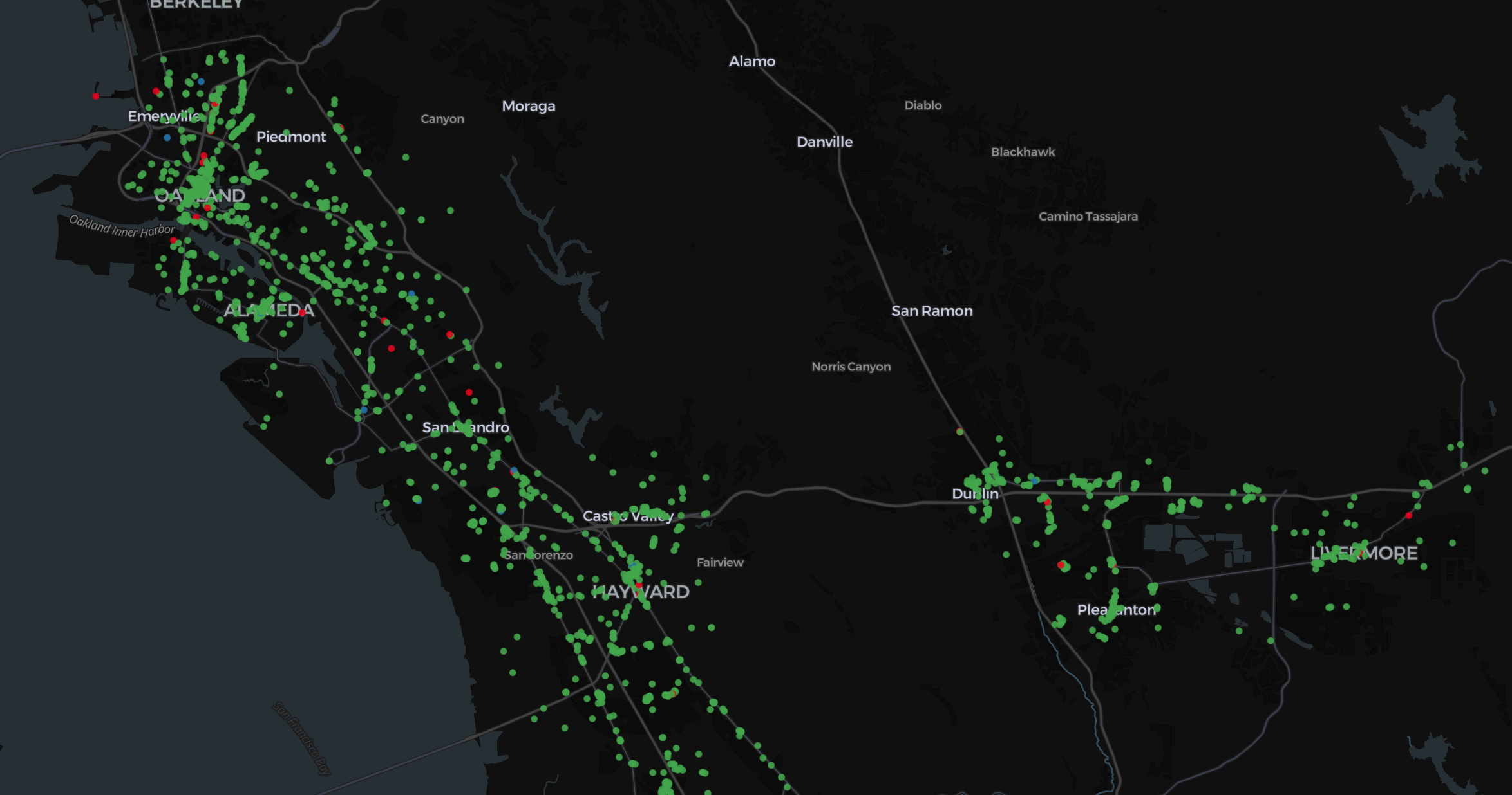
Our matched Overture places, colored by their most recent inspection rating. Mostly green, thankfully!
I was pleasantly surprised by the ease of embedding matching. There’s a lot to like:
- It’s easy to stand up: All you have to know about your data is what columns you’ll join to generate the input strings. No testing and checking to figure out SQL condition statements. For small, unfamiliar datasets, I’ll definitely be starting with embeddings. Especially if I just need a quick, rough join.
- It matched 10% of the records missed by our complex SQL: Even when we spent the time to get to know the data and create a few conditionals, embedding distances caught a significant amount of our misses. I can see it always being a final step for the stubborn remainders.
- The hardest part is first-time set-up: Most of our time spent generating and comparing embeddings (besides compute time) was getting Ollama set up and finding a model. But Ollama makes that pretty easy and it’s a one-time task.
- There’s certainly room for improvement with embeddings: I didn’t put much thought into picking an embedding model; I just grabbed the largest model in Ollama’s directory with ‘embedding’ in the name. Perhaps a smaller model, like
[nomic-embed-text][nomic]performs just as well asmxbai-embed-large, in a fraction of the time. And these are both general models! Fine-tuning a model to match place names and their addresses could reduce our error rate significantly. And hey: get DuckDB VSS up and running and comparisons could get even faster…
Best of all: I ran this all on a local machine. The staging, exploration, and conflation were done with DuckDB, Ollama, H3, Rowboat3, Kepler (for visualization), and some Python. Aside from H3 and generating our bounding box for downloading our Overture subset, we didn’t touch any geospatial functions, reducing our complexity significantly.
-
Near the first PlaceIQ office, there were two different BP gas stations directly across the street from one another, which we always kept in our conflation test data. ↩
-
We’re using “fun” very loosely here! ↩
-
Fathom released Rowboat, a tool for quickly exploring CSVs, just this month. It’s quickly become my first stop after DuckDB for getting to know data. And despite being a webpage, all the analysis runs locally (similar to Kepler). ↩